Plotting cycles

The charge and discharge cycles associated to a given cell-cycling experiment can be loaded form a .mpt file or a set of .DTA files, using the FileManager class. In this page we will present scripts to perform these different tasks:

• Plot the cycles encoded in a .mpt Biologic file

• Plot the cycles encoded in a set of .DTA Gamry files

• Generate a comparison plot of multiple cell-cycling experiments

• Generate a stacked plot of multiple cell-cycling experiments

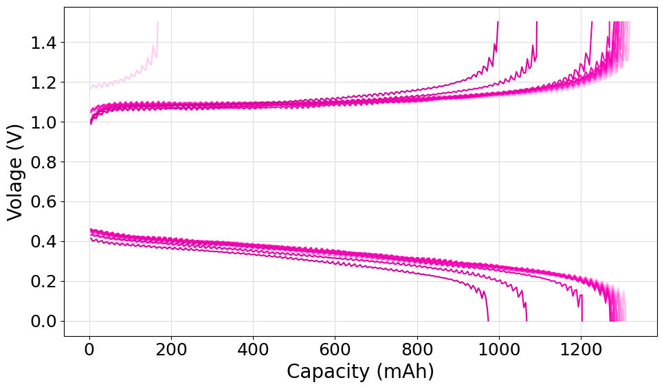
Plot the cycles from a .mpt file

The following script can be used to parse a single .mpt files and plot all the charge and discharge cycles. In the example we demonstrated the use of the fetch_files method of the FileManager class. For the purpose of showing how the operation can be done, we decided to select a subset of cycles to plot (one every 10) and we set the basecolor manually to #FF00BB.

import matplotlib.pyplot as plt
from echemsuite.cellcycling.read_input import FileManager
from echemsuite.graphicaltools import Color, ColorShader

# Read a single .mpt file using the `fetch_files` method
path = "../utils/biologic_single_cycling/biologic_cellcycling.mpt"      # Set here the path to the file
manager = FileManager()
manager.fetch_files([path])
cellcycling = manager.get_cellcycling()

# Select a subset of cycles to be plotted (in this case 1 every 10 cycles)
cycles = [cycle for cycle in cellcycling]
cycles = cycles[::10]

# Define a color for the experiment and setup a shader
basecolor = Color.from_HEX("#FF00BB")
shader = ColorShader(basecolor, len(cycles))

# Create a figure
plt.rcParams.update({'font.size': 18}) 
fig = plt.figure(figsize=(10, 6))

# Plot all the cycles
for i, cycle in enumerate(cycles):

    if cycle.charge and cycle.discharge:
        plt.plot(cycle.charge.Q, cycle.charge.voltage, c=shader[i].RGB)
        plt.plot(cycle.discharge.Q, cycle.discharge.voltage, c=shader[i].RGB)

# Set some properties of the plot
plt.xlabel("Capacity (mAh)", size=20)
plt.ylabel("Volage (V)", size=20)
plt.grid(which="major", c="#DDDDDD")
plt.grid(which="minor", c="#EEEEEE")

# Show the obtained plot
plt.tight_layout()
plt.show()

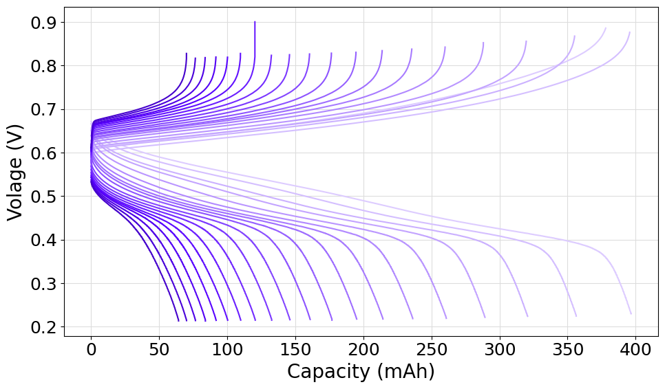
Plot the cycles from a set of .DTA files

The following script can be used to parse multiple .DTA charge/discharge files and plot all cycles. In the example we demonstrated the use of the fetch_from_folder method of the FileManager class to parse all the files in the given folder. For the purpose of showing how the operation can be done, we decided to select the basecolor of the shader from the prism color palette.

import matplotlib.pyplot as plt
from echemsuite.cellcycling.read_input import FileManager
from echemsuite.graphicaltools import ColorShader, Palette

# Read a single set of .DTA files using the `fetch_from_folder` method
path = "../utils/gamry_cellcycling/step_0,1A/CHARGE_DISCHARGE"      # Set here the path to the folder containing the files
manager = FileManager()
manager.fetch_from_folder(path, extension=".DTA")
cellcycling = manager.get_cellcycling()

# Define a color for the experiment and setup a shader
palette = Palette("prism")
shader = ColorShader(palette[0], len(cellcycling))

# Create a figure
plt.rcParams.update({'font.size': 18}) 
fig = plt.figure(figsize=(10, 6))

# Plot all the cycles
for i, cycle in enumerate(cellcycling):

    if cycle.charge and cycle.discharge:
        plt.plot(cycle.charge.Q, cycle.charge.voltage, c=shader[i].RGB)
        plt.plot(cycle.discharge.Q, cycle.discharge.voltage, c=shader[i].RGB)

# Set some properties of the plot
plt.xlabel("Capacity (mAh)", size=20)
plt.ylabel("Volage (V)", size=20)
plt.grid(which="major", c="#DDDDDD")
plt.grid(which="minor", c="#EEEEEE")

# Show the obtained plot
plt.tight_layout()
plt.show()

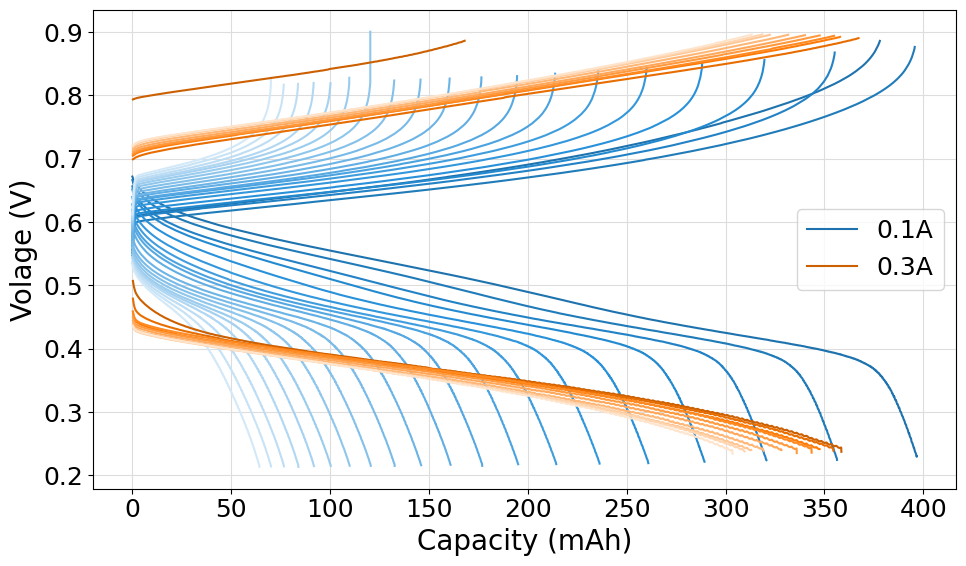
Comparison plot of multiple cell-cycling experiments

The following script can be used to plot multiple cell-cycing experiments on the same plot. An helper function has been defined to help the process of loading files from different folders. We made full use of the Palette and ColorShade class to generate the required color patterns.

import matplotlib.pyplot as plt
from echemsuite.cellcycling.read_input import FileManager
from echemsuite.cellcycling.cycles import CellCycling
from echemsuite.graphicaltools import ColorShader, Palette

# Simple helper function defined to load a cellcycling experiment in a single line
def quickload_folder(folder: str, extension: str) -> CellCycling:
    manager = FileManager()
    manager.fetch_from_folder(folder, extension)
    cellcycling = manager.get_cellcycling()
    return cellcycling

# Define a dictionary encoding the name of the experiment and the corresponding cellcycling object
experiments = {}
experiments["0.1A"] = quickload_folder("../utils/gamry_cellcycling/step_0,1A/CHARGE_DISCHARGE", ".DTA")
experiments["0.3A"] = quickload_folder("../utils/gamry_cellcycling/step_0,3A/CHARGE_DISCHARGE", ".DTA")

# Select a color palette and set the font size
palette = Palette("matplotlib")
plt.rcParams.update({'font.size': 18}) 

# Define a set of subplots (axes will be a tuple of matplotlib axis objects)
fig = plt.figure(figsize=(10, 6))

# Iterate over each experiment and plot all cycles
for i, (name, cellcycling) in enumerate(experiments.items()):
    
    # Set up a color shader based on the palette
    shader = ColorShader(palette[i], len(cellcycling), saturate=True, reversed=True)
    
    # Iterate over all cycles and plot them. Add a legend entry only for the first trace plotted to avoid clutter.
    has_label = False
    for i, cycle in enumerate(cellcycling):

        if cycle.charge and cycle.discharge:
            plt.plot(cycle.charge.Q, cycle.charge.voltage, c=shader[i].RGB, label=name if has_label is False else None)
            plt.plot(cycle.discharge.Q, cycle.discharge.voltage, c=shader[i].RGB)   
            has_label = True

# Render the legend
plt.legend()

# Set the x lable of the last subsplot
plt.xlabel("Capacity (mAh)", size=20)
plt.ylabel("Volage (V)", size=20)
plt.grid(which="major", c="#DDDDDD")
plt.grid(which="minor", c="#EEEEEE")

# Show the obtained plot
plt.tight_layout()
plt.show()

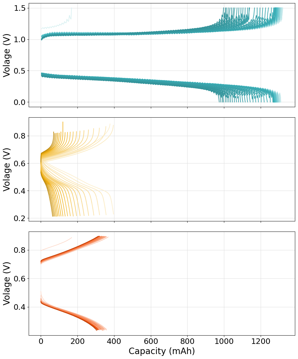
Stacked plot of multiple cell-cycling experiments

The following script can be used to plot multiple cell-cycing experiments on different stacked subsplots. An helper function has been defined to help the process of loading files from different folders. Please notice how both .mpt files and .DTA ones have been loaded in the same script without any issue. We made full use of the Palette and ColorShade class to generate the required color patterns.

import matplotlib.pyplot as plt
from echemsuite.cellcycling.read_input import FileManager
from echemsuite.cellcycling.cycles import CellCycling
from echemsuite.graphicaltools import ColorShader, Palette

# Simple helper function defined to load a cellcycling experiment in a single line
def quickload_folder(folder: str, extension: str) -> CellCycling:
    manager = FileManager()
    manager.fetch_from_folder(folder, extension)
    cellcycling = manager.get_cellcycling()
    return cellcycling

# Define a dictionary encoding the name of the experiment and the corresponding cellcycling object
experiments = {}
experiments["Experiment A"] = quickload_folder("../utils/biologic_single_cycling", ".mpt")
experiments["Experiment B"] = quickload_folder("../utils/gamry_cellcycling/step_0,1A/CHARGE_DISCHARGE", ".DTA")
experiments["Experiment C"] = quickload_folder("../utils/gamry_cellcycling/step_0,3A/CHARGE_DISCHARGE", ".DTA")

# Select a color palette and set the font size
palette = Palette("pastel")
plt.rcParams.update({'font.size': 18}) 

# Define a set of subplots (axes will be a tuple of matplotlib axis objects)
fig, axes = plt.subplots(nrows=len(experiments), figsize=(10, 12))

# Iterate over each experiment and plot all cycles
for i, (name, cellcycling) in enumerate(experiments.items()):
    
    # Extract the current set of axis and setup a color shader based on the palette
    ax = axes[i]
    shader = ColorShader(palette[i], len(cellcycling), saturate=True)
    
    # Iterate over all cycles and plot them
    for i, cycle in enumerate(cellcycling):

        if cycle.charge and cycle.discharge:
            ax.plot(cycle.charge.Q, cycle.charge.voltage, c=shader[i].RGB)
            ax.plot(cycle.discharge.Q, cycle.discharge.voltage, c=shader[i].RGB)

    # Add a y label and to each subsplot and add a grid
    ax.set_ylabel("Volage (V)", size=20)
    ax.grid(which="major", c="#DDDDDD")
    ax.grid(which="minor", c="#EEEEEE")

# Set the x lable of the last subsplot
axes[-1].set_xlabel("Capacity (mAh)", size=20)

# Show the obtained plot
plt.tight_layout()
plt.show()

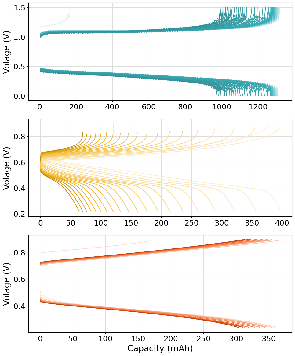
Please notice how the subplots generated have different x-axis scales. If the same scale must be applied to each subplot in order to be directly “vertically” comparable, the sharex="all" option should be used in the fig, axes = plt.subplots(nrows=len(experiments), figsize=(10, 14)) instruction. The resulting plot will appears as: